Finding Similar Trajectories
This post is about finding and analysing similar trajectories using Traffic-flow data as a real world example. We aim to find meaningful relationship between different trajectories in our data. Then we plan to use them for forecasting in the next blogpost.
Intro
I gave brief information about the data and did some cleaning/preperation in the previous post. Now I will talk about distance functions and use them for capturing patterns/similarities in our data.
Split
Before that, I split data to 2 main parts training and testing. Also I split each part to two smaller intersecting parts which I call reference and query. There is no need to explain train/test splitting, the reference and query parts are because of the way searching for historical similarity works, which I will tell right after showing the split.

Split Visual
Note that, query and reference parts are intersecting with each other. When searching for similar trajectories, we need to use data from past otherwise the first entries of the query part would have nowhere to look. As an example, if we were only using October 2021 to February 2022 in training, first weeks of October 2021 would only be searching the same days and maybe weeks for similar patterns. With query/reference split I create a year long pool to search for similar patterns. This also lets me to capture a possible yearly pattern.
Also, I see that the flow data changes drastically right before 2021. This makes 4+12 months of split a viable option, using a bigger set may create problems.
Workflow
- The procedure summary:
- Arrange the time-series data to overlapping small windows(vectors/trajectories).
- Use distance functions to find similar trajectories for each trajectory.
- Observe that: windowsize and distance functions (and also number of similar trajectories to be analysed) are all parameters that we should take care of
- Windowsize:
- should be large enough to capture an ongoing pattern, but small
enough to be relatable
- e.g. using a windowsize of 24 hours would not be very helpful as everyday is similar to each other and knowing such similar trajectories would not be helpful for making a forecast
- should be large enough to capture an ongoing pattern, but small
enough to be relatable
Arranging Data to Trajectory Format
For capturing trajectory similarities, we first need trajectories. I arrange the time-series data to overlapping small windows (vectors/trajectories). The lenght(size) of these windows are of great interest. I will be calling it windowsize in this and following posts.
Windowsize should be large enough to capture an ongoing pattern but small enough to be relateble. As an example, 4 hour long trajectory gives strong clues about the time of the day, trend of the traffic and that specific days average flow. Using 24 hour would may give better information about that day but it would miss time of the day and other critical information.
Distance Functions
When windowed data arrangement is done, I use distance functions to find closest windows for each window. This functions are usually metrics, but it is not necessary. I first talk about the basic metrics. Then I may talk about custom made distance functions that fit better for my purpose. I leave explaining the details of each distance to below chart from Shirkhorshidi et. al., I will only talk about some insights about the measures I will use.
.png)
Euclidean Distance
Euclidean (or \(\ell^2\)) distance is an obvious choice for measuring distance. It is widespread and easy to implement/understand.
In our case, euclidean distance gives easy to understand results. If two trajectories are similar according to euclidean distance, we can confidently say they are indeed similar. However it has some of shortcomings. Here are some of them with possible solutions.
A single steep anomaly may disrupt the whole measure (especially right before/after rush hours)
Smoothen the outlier values
Ignore some of the elements in the trajectory
Past values may affect the result by a lot
Weight the latter elements more (weighted euclidean)
other distances are just a sketch for now. no need to discuss them a lot imho
Manhattan Distance
Similar to Euclidean
Maximum Distance
Very easy to implement
Very fast
not expected to work as well as euclidean (however it performed ok, check next post)
Correlation Distance
may catch different patterns compared to above three.
may miss many important patterns too
Coding
will add.
Analysis
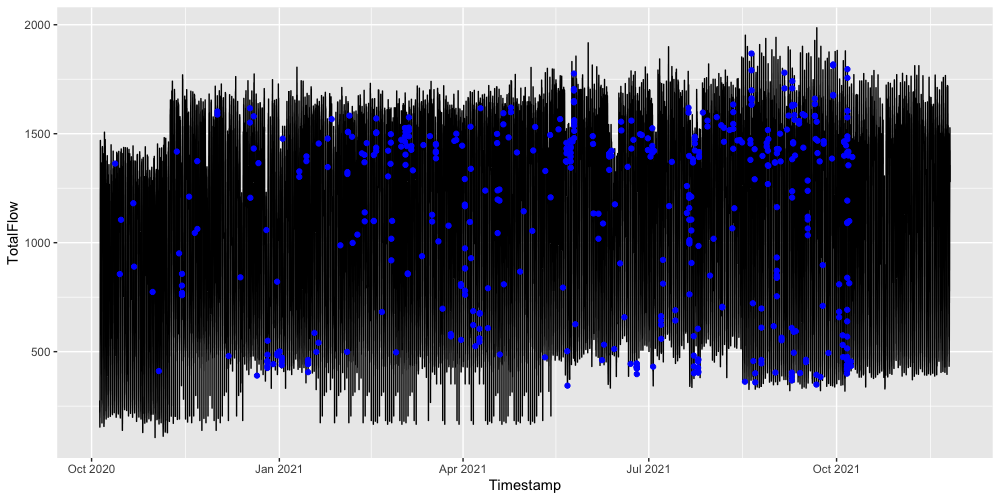
Inspecting the closest neighbors gives a more or less uniform distribution.
Here are two example visuals showing the nearest (only the first one) neighbor of first 500 observations from the query(train) set. (500 observations are about 5 days long)

Windowsize = 10, 5 days
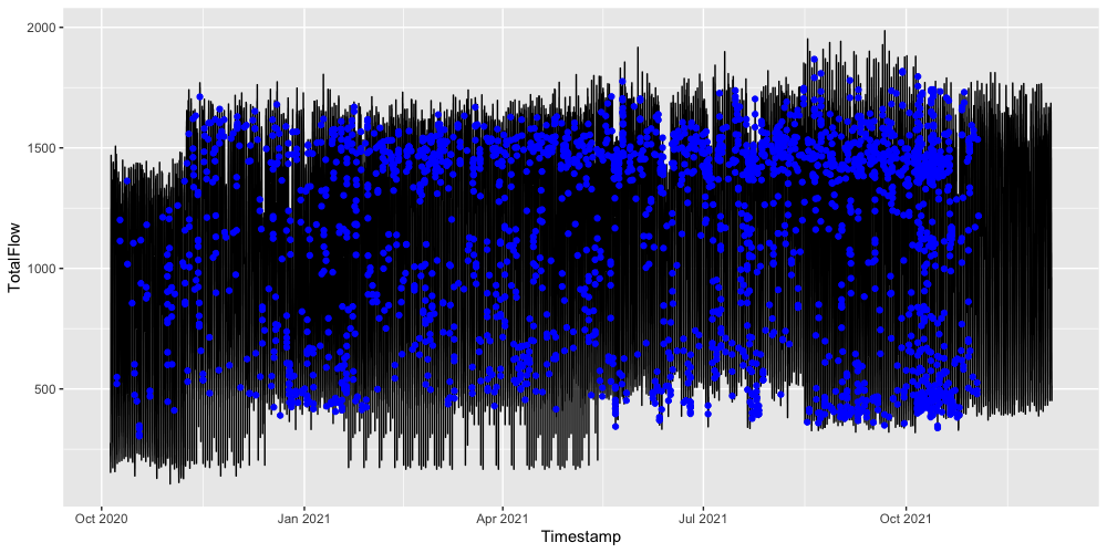
Also increasing 5 days to 1 month, we see similar results.

Windowsize 10, 1 month
In both examples there is uniform-like patterns. I checked different statistics like
- How many times does an observation is the closest neighbor?
- Is there a relationship between similar hours? (yes but not as much as expected) (i may add it too in future)
- etc.
These results suggests verifies our choice of using long time-span. Thus in the next post, I will be using the nearest neighbors for making forecasts on the full size data without any extra touch.