Explanatory Data Analysis on Traffic Data
Data Description
I use traffic flow data from California Freeway Performance Measure Systems (PeMS). The dataset spans on years and contains huge number of stations (that correspond to different highways/streets etc.). I select around two years of timespan from October 2020 to June 2022. I will show three different stations with varying occupancies in this post.
The data contains various statistics such as total traffic flow of 5 minute intervals, average speed and occupancy. I will be only interested in total traffic flow of 15 minute intervals. The reasoning behind 15 minutes is discussed in many papers like Lippi. Briefly, 15 minute is a good trade-off between reducing the noise with keeping the data relatable and useful.
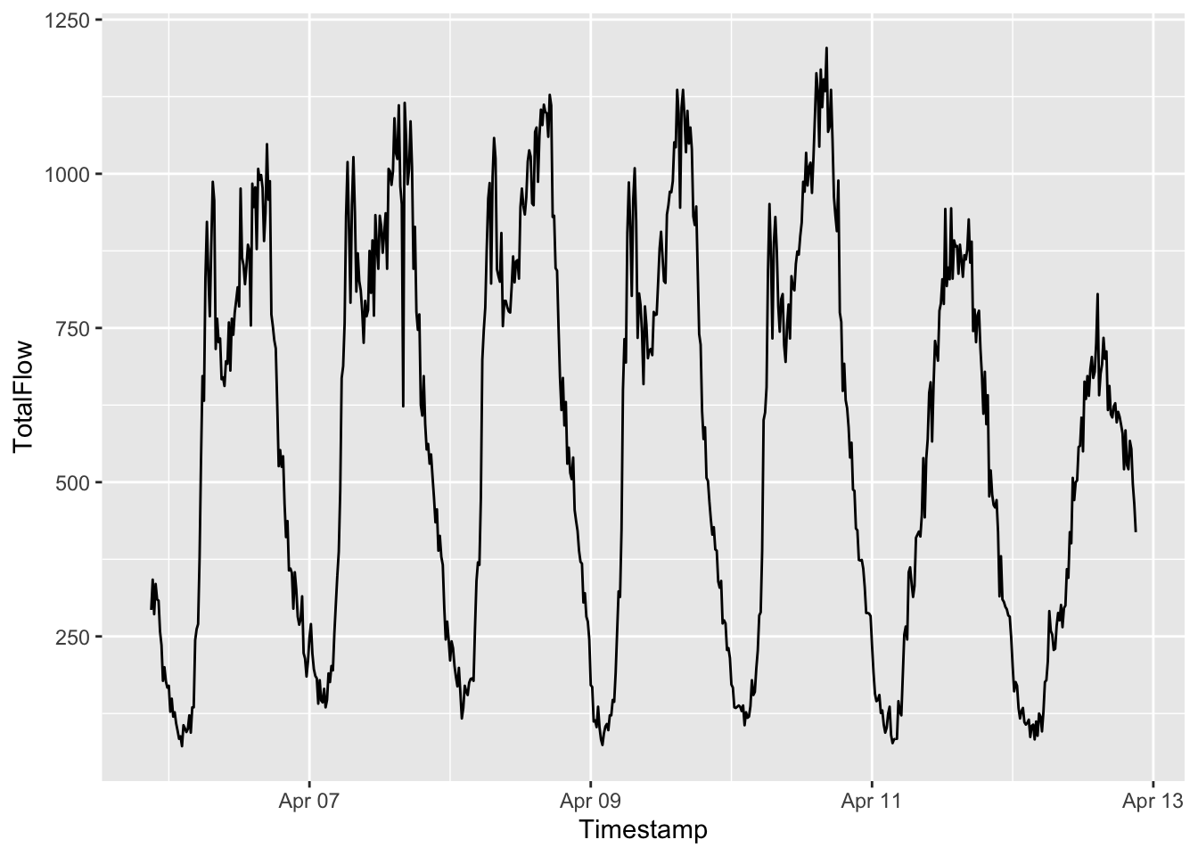
Here is a one week look to the data:

It is clear that weekdays and weekends look different. This lead people to use only weekends in their projects especially for capturing seasonal (daily) patterns.
Missing Data
Using this data as an example, I will show a way to find missing dates in huge datasets.
In PeMS data there were some dates with no observations, however their dates were also not included. Thus we need to find the dates that do not appear in the data to find the missing observations.
library(lubridate)

# create all dates along the data.
alldates = seq(ymd_hm('2020-04-01 00:00'), ymd_hm('2022-06-04 23:55 '), by = '5 mins')

# create a checker
bigdates = data.table(Timestamp = alldates,
                      isempty = 0)

# merge the checker with the data of interest
bigdates = merge(bigdates,
                 data %>% filter(Timestamp < "2022-06-03"),
                 all = TRUE,
                 by = "Timestamp")

# the NA values in the merge dataset are the non-existing ones.
bigdates[which(is.na(bigdates$Station)), ]$Timestamp
I did not include the results, but there were some instances of missing data. I handled them with two methods:
- When missing data is not consecutive, I used the flow from one week
before
- To be precise: \((60/5) \times 24 \times 7 = 2016\) rows above.
- In February 6 2022, there was couple hours long of missing data. I took average of same day/hour flow from the previous 3 weeks to fill the missing values.
Here is a custom (and weird) function for the second case. Even though it was simple to explain, working with time data may be tricky. In my case UTC was not stable in different runs. Also, I did not want to work with indices because of some other problems that I don’t recall.
missing_replacer_3week <- function(data, year = 2022, month = 2, mday = 5, hour, minute, year1 = 2022, month1 = 1, mday1 = 29, year2 = 2022, month2 = 1, mday2 = 22, year3 = 2022, month3 = 1, mday3 = 15) {
    xxx = rbind(data[year(Timestamp) %in% year1 & month(Timestamp) == month1 & mday(Timestamp) == mday1 & hour(Timestamp) == hour & minute(Timestamp) == minute, 8:13],
                data[year(Timestamp) %in% year2 & month(Timestamp) == month2 & mday(Timestamp) == mday2 & hour(Timestamp) == hour & minute(Timestamp) == minute, 8:13],
                data[year(Timestamp) %in% year3 & month(Timestamp) == month3 & mday(Timestamp) == mday3 & hour(Timestamp) == hour & minute(Timestamp) == minute, 8:13])
    xxx = data.table(t(apply(xxx, 2, mean)))
    data[year(Timestamp) == year & month(Timestamp) == month & mday(Timestamp) == mday & hour(Timestamp) == hour & minute(Timestamp) == minute, 8:13] =
        xxx
    data[year(Timestamp) == year & month(Timestamp) == month & mday(Timestamp) == mday & hour(Timestamp) == hour & minute(Timestamp) == minute, 3:7] =
        data[year(Timestamp) %in% year1 & month(Timestamp) == month1 & mday(Timestamp) == mday1 & hour(Timestamp) == hour & minute(Timestamp) == minute, 3:7]
    return(data)
}
Next Post
This post was a short introduction. After preparing the data, I started working on similar trajectories.