Combining Quantile Forecasts
Note that this is the third post of a three post series about Quantile Forecast Models. The first two posts are still being prepared. The first post will be about QR and examples from
R. The second one will define QRA. If you want to learn more about QRA before reading this post, there may not be a simple tutorial online but you can check the paper from the founders of QRA.
QRA is a great tool for combining forecasts and creating a quantile model but it can only be used when combining “Point Forecast Models”. That arises the question:
What to do when we want to combine “Quantile Forecast Models”?
In this article I will walk you through 9 different methods for combining quantile forecasts (maybe with examples using R).
For that, let’s first assume we have 5 different quantile forecast models at 4 different quantiles:
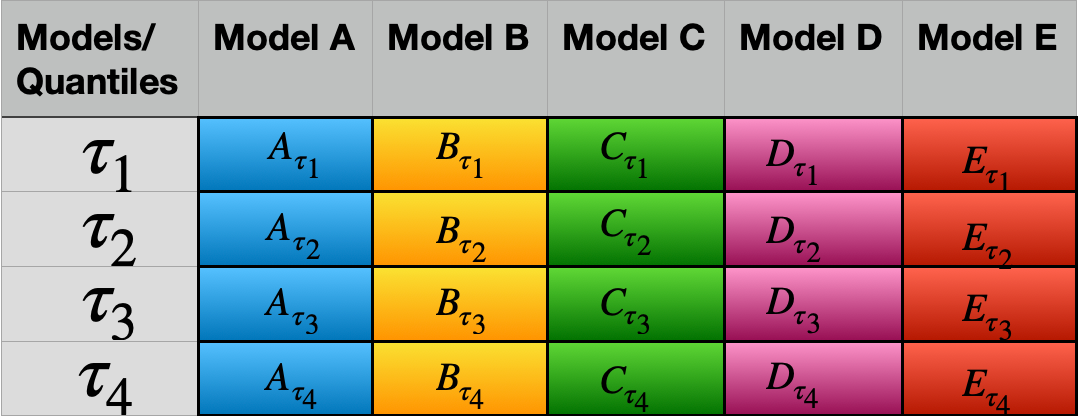
Quantile predictions from 5 models at 4 different quantiles
Note that we want to combine these results to create a better model. Let M be our new model and we want to find:

Let’s see some different approaches:
Naive Method
We have 5 different models and in every model 4 different quantile results. For simplicity, just think these results as 20 individual results.

All results.
Sort the results in ascending order.

Results mixed then sorted in ascending order.
Then the Naive approach says: “Take every 5th (greatest element for each group with N(5) elements) element and assign it to a quantile in ascending order”:
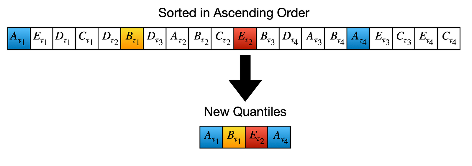
The Combined Model has new quantile values.
So we can finalize our naive model with the results:
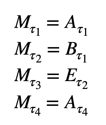
Results of the Naive Method
Median Value Method
We take the median for each 5 (N) element group. These medians are assigned as the quantile results of the new combined model.
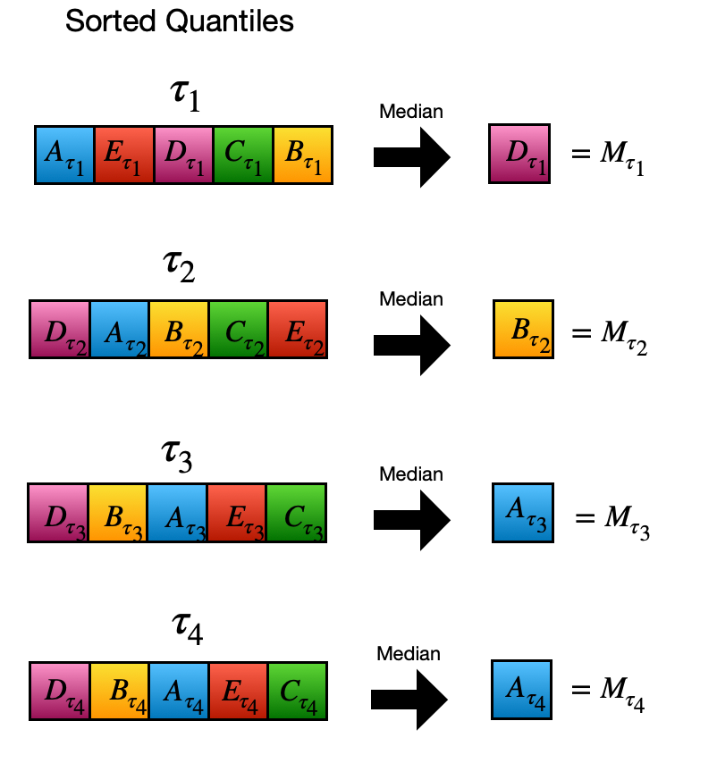
For new quantiles, median from each quantile group is chosen.
Simple Averaging
Again results are grouped by 5 elements. This time we take the average (mean) instead of median:
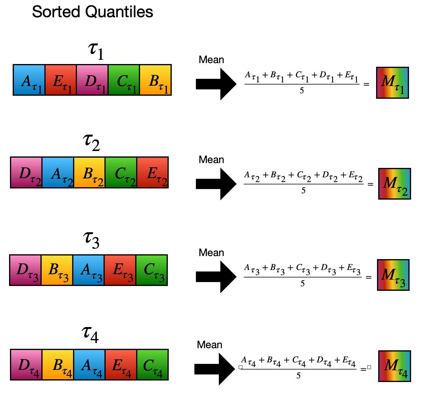
Weighted Averaging
It is very similar to weighted averaging. However, this time each result is weighted corresponding to their accuracy. The accuracy comparison can be done in many different ways and left beyond the scope of this article.
QRA-E
Things get interesting from now on, so be careful about every step, some steps will seem weird until you see the whole picture.
We again sort our mixed results. Then we take mean of every 5 element group and think them as “point forecast” results of new “made up” models.
We will use these models for creating the “combined quantile model”.
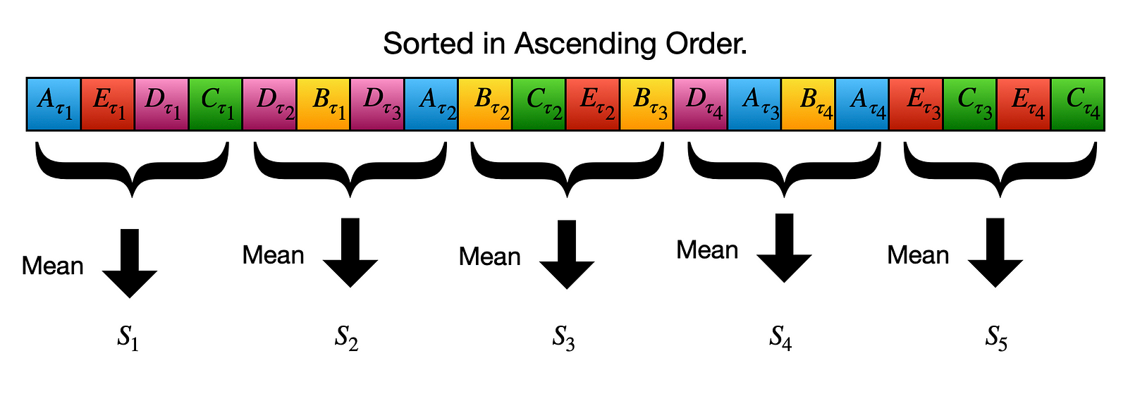
Mean of every 5 element group is assigned as a point forecast of a new “made up” model.
Note that, these models are far from being accurate. Surely, we know that S1 model underestimates and S5 model overestimates. However, we won’t be using them alone. We will be using these unaccurate “point forecast” models as inputs of a new QRA model.
The reasoning behind these “bad” forecasts can be seen easily. As we are planning to make a quantile prediction, having underestimating and overestimating models will be useful. Also in this method we are able to change the number of quantiles we want as an output, contrary to previous methods.
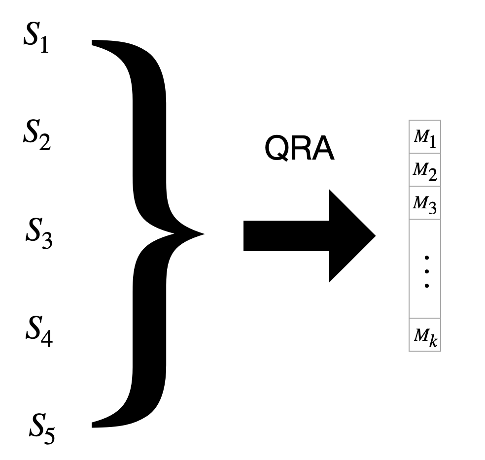
Using made up forecast results as features in QRA.
A very brief summary: Here, we first some created “bad” point forecast models then used them in QRA.
QRA-A
This is very similar to QRA-E, but instead of grouping results and creating 5 models, now we create 100 models with thinking every individual result as a point forecast result.
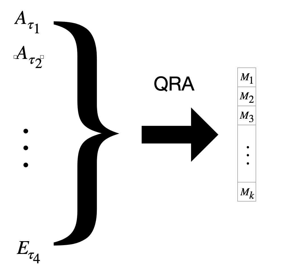
Thinking each quantile result from each model as an individual result. Then using it as a feature in QRA.
QRA-T
This is again very similar to QRA-A. However, this time we will be “targeting” some quantiles when choosing the results we are putting in QRA.
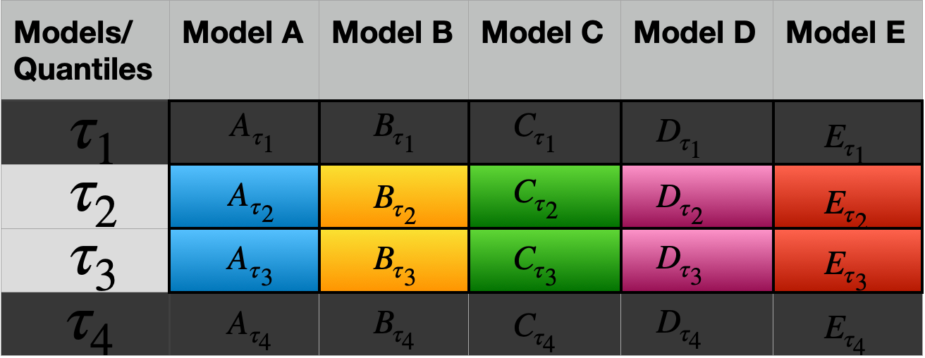
Here we choose second and third quantiles.
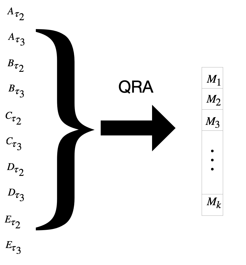
Very similar to QRA-A, we put all results from “targeted”(selected) quantiles to QRA.
Note about QRA-E/A/T
You can see that we are choosing different number of forecasts in each method. This means that the number of features used in each QRA model differs.
Recall: Pinball Loss Function
Let’s recall the Pinball Loss Function that we have explained in Quantile Regression article:
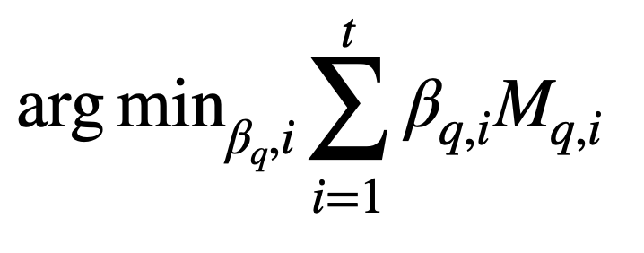
For every quantile, q, we are trying to minimize that loss function.
We won’t be going in much detail here but that recalling that function will be useful in the following sections.
Constrained QRA-E (CQRA-E)
The only difference between CQRA-E and QRA-E is the added constraints in the loss function:
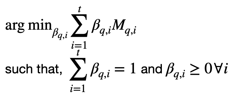
Loss function with constraints.
With that constraints, the aim is to take “literally” weighted average(?) of every model instead of having negative coefficients for some models while having very big positive coefficients for others.
The reasoning for this is understandable:
Having negative coefficients for model combination does not make a lot of sense in our situation. The reasoning is the model results are different from other features, they all are an approximation to the real result.
Constrained QRA-A (CQRA-A)
This has the same logic as the CQRA-E. This time these constrains are added to the QRA-A method.
Constrained QRA-T (CQRA-T)
This is again the same, but done on CQRA-T. However this outperforms the other two methods. We will try to understand the reason now.
Results
Excessive constraints of CQRA-E reduces the performance. Only selecting a few of the values with CQRA-T solves this problem and gives great results.